
This week, I had the opportunity to present R data.table package to R Ladies Twin Cities meetup. With the help of another R Lady, Haema Nilakanta, we put together this tutorial on the package. This document was originally published on RPubs here.
This document is by no means exhaustive. However, it is a good start for those who would like to get introduced to data.table.
Overview
What is data.table?
“data.table is an R package that provides an enhanced version of data.frames.” It provides a faster and more efficient way to do data manipulation while drastically reducing the amount of memory required. It’s an excellent addition to your R venacular, particularly if you work with massive datasets.
Install and load
# install
install.packages("data.table")
# load
library(data.table)
The Basics
A lot of data.table commands are similar to the usual R data.frame. For example, you can create a data.table similar to how you create a new data.frame.
# create a data.table
DT <- data.table(x = c(1, 2, 3), y = c('a', 'b', 'c'))

# turn iris data.frame to a data.table object
data("iris")
iris_dt <- as.data.table(iris)
# setDT(iris) # turn iris into a data.table instead of making a copy
# print
iris_dt
## Sepal.Length Sepal.Width Petal.Length Petal.Width Species
## 1: 5.1 3.5 1.4 0.2 setosa
## 2: 4.9 3.0 1.4 0.2 setosa
## 3: 4.7 3.2 1.3 0.2 setosa
## 4: 4.6 3.1 1.5 0.2 setosa
## 5: 5.0 3.6 1.4 0.2 setosa
## ---
## 146: 6.7 3.0 5.2 2.3 virginica
## 147: 6.3 2.5 5.0 1.9 virginica
## 148: 6.5 3.0 5.2 2.0 virginica
## 149: 6.2 3.4 5.4 2.3 virginica
## 150: 5.9 3.0 5.1 1.8 virginicaWhen a data.table has more than 100 rows, it automatically prints the first five and the last five rows.
Subset
Select first 3 rows:
# data.frame
iris[1:3,]
## Sepal.Length Sepal.Width Petal.Length Petal.Width Species
## 1 5.1 3.5 1.4 0.2 setosa
## 2 4.9 3.0 1.4 0.2 setosa
## 3 4.7 3.2 1.3 0.2 setosa# data.table
iris_dt[1:3]## Sepal.Length Sepal.Width Petal.Length Petal.Width Species
## 1: 5.1 3.5 1.4 0.2 setosa
## 2: 4.9 3.0 1.4 0.2 setosa
## 3: 4.7 3.2 1.3 0.2 setosaFind rows where Species == "setosa":
# data.frame
iris[iris$Species == "setosa",]
# data.table
iris_dt[Species == "setosa"]
Find rows where Species == "setosa" and Sepal.Length == 5:
# data.frame
iris[iris$Species == "setosa" & iris$Sepal.Length == 5,]
# data.table
iris_dt[Species == "setosa" & Sepal.Length == 5]
# advanced data.table
tmp <- data.table(Species = "setosa", Sepal.Length = 5, key = c("Species", "Sepal.Length"))
setkey(iris_dt, Species, Sepal.Length)
iris_dt[tmp]
Notice with the usual data.frame, you end up calling the dataset multiple times, once to get the column information and every time a column is referenced. Meanwhile in the data.table package, you only need to refer to the dataset once.
Manipulation on Columns and Group By
Select subset of columns:
# data.frame
iris[, c("Species", "Petal.Width", "Petal.Length")]
# data.table
iris_dt[, .(Species, Petal.Width, Petal.Length)]
Calculate the mean value of Sepal.Length:
# data.frame
mean(iris$Sepal.Length)
## [1] 5.843333# data.table
iris_dt[, mean(Sepal.Length)]## [1] 5.843333One major advantage of data.table is it can aggregate data with the table setting. For example, instead of using the aggregate function to compute the mean Sepal.Length by Species, we can do this directly in the iris_dt. This saves us a good chunk of time especially when we have a lot of rows to take a function over.
# data.frame
aggregate(Sepal.Length ~ Species, iris, mean) # no easy way to do this in base R
## Species Sepal.Length
## 1 setosa 5.006
## 2 versicolor 5.936
## 3 virginica 6.588# data.table
iris_dt[, mean(Sepal.Length), by = .(Species)]## Species V1
## 1: setosa 5.006
## 2: versicolor 5.936
## 3: virginica 6.588The data.table syntax of .() basically calls on certain columns.
Consider now we only want to calculate mean Sepal.Length by Species where Sepal.Width >= 3, instead of first having to subset the entire dataset and then running the function we can do this in one step and create a new variable called mean_sepal_length.
# data.frame
aggregate(Sepal.Length ~ Species, iris[iris$Sepal.Width >= 3,], mean)
## Species Sepal.Length
## 1 setosa 5.029167
## 2 versicolor 6.218750
## 3 virginica 6.768966# data.table
iris_dt[Sepal.Width >= 3, .(mean_sepal_length = mean(Sepal.Length)), by = .(Species)]## Species mean_sepal_length
## 1: setosa 5.029167
## 2: versicolor 6.218750
## 3: virginica 6.768966You can also use expressions within by statement. For example, calculate mean sepal length for Sepal.Width > 3 and Sepal.Width <= 3:
iris_dt[, mean(Sepal.Length), by = .(width_larger_than_3 = Sepal.Width > 3)]## width_larger_than_3 V1
## 1: TRUE 5.683582
## 2: FALSE 5.972289Another powerful tool of this package is the .N command. This is a counting tool that holds the number of observations in the current group. For example, if we want to calculate the number of rows:
# data.frame
nrow(iris)
## [1] 150# data.table
iris_dt[, .N]## [1] 150Or calculate number of unique values for Species:
# data.frame
length(unique(iris$Species))
## [1] 3# data.table
iris_dt[, uniqueN(Species)]## [1] 3Or calculate number of observations by Species:
# data.frame
data.frame(table(iris$Species))
## Var1 Freq
## 1 setosa 50
## 2 versicolor 50
## 3 virginica 50# data.table
iris_dt[, .N, Species]## Species N
## 1: setosa 50
## 2: versicolor 50
## 3: virginica 50Multiple operations in one go: calculate mean and number of operations by Species
# data.table
iris_dt[, .(mean_sepal_length = mean(Sepal.Length), no_obs = .N), by = .(Species)]
## Species mean_sepal_length no_obs
## 1: setosa 5.006 50
## 2: versicolor 5.936 50
## 3: virginica 6.588 50A similar command to .N is .I which holds the row numbers, and can be assigned to a variable.
# return row numbers
iris_dt[, .I]
## [1] 1 2 3 4 5 6 7 8 9 10 11 12 13 14 15 16 17
## [18] 18 19 20 21 22 23 24 25 26 27 28 29 30 31 32 33 34
## [35] 35 36 37 38 39 40 41 42 43 44 45 46 47 48 49 50 51
## [52] 52 53 54 55 56 57 58 59 60 61 62 63 64 65 66 67 68
## [69] 69 70 71 72 73 74 75 76 77 78 79 80 81 82 83 84 85
## [86] 86 87 88 89 90 91 92 93 94 95 96 97 98 99 100 101 102
## [103] 103 104 105 106 107 108 109 110 111 112 113 114 115 116 117 118 119
## [120] 120 121 122 123 124 125 126 127 128 129 130 131 132 133 134 135 136
## [137] 137 138 139 140 141 142 143 144 145 146 147 148 149 150# assign row numbers to variable row_id
iris_dt[, row_id := .I]
head(iris_dt, 3)## Sepal.Length Sepal.Width Petal.Length Petal.Width Species row_id
## 1: 5.1 3.5 1.4 0.2 setosa 1
## 2: 4.9 3.0 1.4 0.2 setosa 2
## 3: 4.7 3.2 1.3 0.2 setosa 3.GRP command allows you to add unique id to groups as identified by by statement.
iris_dt[, .GRP]## [1] 1iris_dt[, .GRP, by = .(Species, sepal_width_larger_than_3 = Sepal.Width > 3)]## Species sepal_width_larger_than_3 GRP
## 1: setosa TRUE 1
## 2: setosa FALSE 2
## 3: versicolor TRUE 3
## 4: versicolor FALSE 4
## 5: virginica TRUE 5
## 6: virginica FALSE 6Keys
Once you get more comfortable with data.table, you can start to take advantage of its unique options. One way to really speed up your use of a large dataset is by setting the key(s). This allows the merging of multiple datasets or subsetting to go much faster. data.tables are also sorted by their keys.
Sort by Species and Sepal.Length:
# data.frame
iris[with(iris, order(Species, Sepal.Length)), ]
# data.table
iris_dt[order(Species, Sepal.Length)] # does not store the ordering, unless assign to a variable name
setkey(iris_dt, Species, Sepal.Length) # keys are added; data.table is always sorted by its key columns
Calculate mean Sepal.Width by Species and order the results by Species:
# data.frame
tmp_iris <- aggregate(Sepal.Width ~ Species, iris, mean)
tmp_iris[with(tmp_iris, order(Species)),]
# data.table
iris_dt[, .(mean_sepal_width = mean(Sepal.Width)), keyby = .(Species)]
If it is not necessary to keep the original ordering of the variable(s) in by statement, using keyby can speed up even more. And the resulting data.table is sorted by the variable(s) in the keyby statement.
Joins
Inner join two data.tables:
dt1 <- data.table(x = c(1, 2, 3), y = c("a", "b", "c"), key = c("y"))
dt2 <- data.table(y = c("a", "c", "d", "e"), z = c(10, 20, 30, 40), key = c("y"))
dt1[dt2, nomatch = 0]
## x y z
## 1: 1 a 10
## 2: 3 c 20# or
dt1[dt2, on = .(y), nomatch = 0] # equi: merge(dt1, dt2)on needs to be specified if no keys are set, or if dt1 and dt2 do not have the exact same keys, or if you want to join the two data.tables using variables other than the keys.
Left/Right joins:
# keep everything from dt2
dt1[dt2, on = .(y)] # equi: merge(dt1, dt2, all.y = TRUE)
## x y z
## 1: 1 a 10
## 2: 3 c 20
## 3: NA d 30
## 4: NA e 40# keep everything from dt1
dt2[dt1, on = .(y)] # equi: merge(dt1, dt2, all.x = TRUE)## y z x
## 1: a 10 1
## 2: b NA 2
## 3: c 20 3Full joins:
merge(dt1, dt2, all = TRUE)## y x z
## 1: a 1 10
## 2: b 2 NA
## 3: c 3 20
## 4: d NA 30
## 5: e NA 40Defining function :=
You can define new variables in data.table with the := function.
# create a new variable called newIris
iris_dt[, newIris := Petal.Width/Petal.Length]
head(iris_dt, 3)
## Sepal.Length Sepal.Width Petal.Length Petal.Width Species row_id
## 1: 5.1 3.5 1.4 0.2 setosa 1
## 2: 4.9 3.0 1.4 0.2 setosa 2
## 3: 4.7 3.2 1.3 0.2 setosa 3
## newIris
## 1: 0.1428571
## 2: 0.1428571
## 3: 0.1538462# create a new variable mean_petal_width by species
iris_dt[, mean_petal_width := mean(Petal.Width), .(Species)]
head(iris_dt, 3)## Sepal.Length Sepal.Width Petal.Length Petal.Width Species row_id
## 1: 5.1 3.5 1.4 0.2 setosa 1
## 2: 4.9 3.0 1.4 0.2 setosa 2
## 3: 4.7 3.2 1.3 0.2 setosa 3
## newIris mean_petal_width
## 1: 0.1428571 0.246
## 2: 0.1428571 0.246
## 3: 0.1538462 0.246Or, you can create multiple variables all in one go
iris_dt[, `:=` (newIris = Petal.Width/Petal.Length,
                row_id = .I)]
# or
iris_dt[, c("newIris", "row_id") := list(Petal.Width/Petal.Length, .I)]
One great benefit of data.table is the ability to sub-assign by reference.
# create a new variable setosa_dummy which equals 1 for setosa species, NA otherwise
iris_dt[Species == "setosa", setosa_dummy := 1]
# rename setosa to renamed_setosa
iris_dt[Species == "setosa", Species := "renamed_setosa"]
head(iris_dt, 3)
## Sepal.Length Sepal.Width Petal.Length Petal.Width Species row_id
## 1: 5.1 3.5 1.4 0.2 renamed_setosa 1
## 2: 4.9 3.0 1.4 0.2 renamed_setosa 2
## 3: 4.7 3.2 1.3 0.2 renamed_setosa 3
## newIris mean_petal_width setosa_dummy
## 1: 0.1428571 0.246 1
## 2: 0.1428571 0.246 1
## 3: 0.1538462 0.246 1You can also use := to remove columns.
# remove newIris column
iris_dt[, newIris := NULL]
# remove mean_petal_width and row_id
iris_dt[, c("mean_petal_width", "row_id", "setosa_dummy") := NULL]
# or
cols <- c("mean_petal_width", "row_id", "setosa_dummy")
iris_dt[, (cols) := NULL]# or
iris_dt[, `:=` (mean_petal_width = NULL, row_id = NULL, setosa_dummy = NULL)]
head(iris_dt, 3)## Sepal.Length Sepal.Width Petal.Length Petal.Width Species
## 1: 5.1 3.5 1.4 0.2 renamed_setosa
## 2: 4.9 3.0 1.4 0.2 renamed_setosa
## 3: 4.7 3.2 1.3 0.2 renamed_setosaMore Advanced
.SD and .SDcols
You can access columns of a data.table using .SD and .SDcols syntax.
Select all columns in iris_dt:
iris_dt[, .SD]## Sepal.Length Sepal.Width Petal.Length Petal.Width Species
## 1: 5.1 3.5 1.4 0.2 renamed_setosa
## 2: 4.9 3.0 1.4 0.2 renamed_setosa
## 3: 4.7 3.2 1.3 0.2 renamed_setosa
## 4: 4.6 3.1 1.5 0.2 renamed_setosa
## 5: 5.0 3.6 1.4 0.2 renamed_setosa
## ---
## 146: 6.7 3.0 5.2 2.3 virginica
## 147: 6.3 2.5 5.0 1.9 virginica
## 148: 6.5 3.0 5.2 2.0 virginica
## 149: 6.2 3.4 5.4 2.3 virginica
## 150: 5.9 3.0 5.1 1.8 virginicaSelect subset of columns by specifying columns in .SDcols:
iris_dt[, .SD, .SDcols = c("Species", "Sepal.Width", "Sepal.Length")]## Species Sepal.Width Sepal.Length
## 1: renamed_setosa 3.5 5.1
## 2: renamed_setosa 3.0 4.9
## 3: renamed_setosa 3.2 4.7
## 4: renamed_setosa 3.1 4.6
## 5: renamed_setosa 3.6 5.0
## ---
## 146: virginica 3.0 6.7
## 147: virginica 2.5 6.3
## 148: virginica 3.0 6.5
## 149: virginica 3.4 6.2
## 150: virginica 3.0 5.9# or
iris_dt[, .SD, .SDcols = c(5,1,2)]## Species Sepal.Length Sepal.Width
## 1: renamed_setosa 5.1 3.5
## 2: renamed_setosa 4.9 3.0
## 3: renamed_setosa 4.7 3.2
## 4: renamed_setosa 4.6 3.1
## 5: renamed_setosa 5.0 3.6
## ---
## 146: virginica 6.7 3.0
## 147: virginica 6.3 2.5
## 148: virginica 6.5 3.0
## 149: virginica 6.2 3.4
## 150: virginica 5.9 3.0Round up all numeric columns to integer:
iris_dt[, lapply(.SD, round), .SDcols = 1:4]## Sepal.Length Sepal.Width Petal.Length Petal.Width
## 1: 5 4 1 0
## 2: 5 3 1 0
## 3: 5 3 1 0
## 4: 5 3 2 0
## 5: 5 4 1 0
## ---
## 146: 7 3 5 2
## 147: 6 2 5 2
## 148: 6 3 5 2
## 149: 6 3 5 2
## 150: 6 3 5 2# assign them to the original columns
cols <- 1:4 # or cols <- c("Sepal.Length", "Sepal.Width", "Petal.Length", "Petal.Width")
iris_dt[, (cols) := lapply(.SD, round), .SDcols = cols]
head(iris_dt, 3)## Sepal.Length Sepal.Width Petal.Length Petal.Width Species
## 1: 5 4 1 0 renamed_setosa
## 2: 5 3 1 0 renamed_setosa
## 3: 5 3 1 0 renamed_setosaCalculate mean by Species:
iris_dt <- as.data.table(iris)
# mean of all columns by Species
iris_dt[, lapply(.SD, mean), by = Species]
## Species Sepal.Length Sepal.Width Petal.Length Petal.Width
## 1: setosa 5.006 3.428 1.462 0.246
## 2: versicolor 5.936 2.770 4.260 1.326
## 3: virginica 6.588 2.974 5.552 2.026# or if we only want to calculate mean of Sepal columns by Species
iris_dt[, lapply(.SD, mean), by = Species, .SDcols = c("Sepal.Length", "Sepal.Width")]## Species Sepal.Length Sepal.Width
## 1: setosa 5.006 3.428
## 2: versicolor 5.936 2.770
## 3: virginica 6.588 2.974Select first and last rows:
iris_dt[, .SD[c(1, .N)]]## Sepal.Length Sepal.Width Petal.Length Petal.Width Species
## 1: 5.1 3.5 1.4 0.2 setosa
## 2: 5.9 3.0 5.1 1.8 virginica# by Species
iris_dt[, .SD[c(1, .N)], by = Species]## Species Sepal.Length Sepal.Width Petal.Length Petal.Width
## 1: setosa 5.1 3.5 1.4 0.2
## 2: setosa 5.0 3.3 1.4 0.2
## 3: versicolor 7.0 3.2 4.7 1.4
## 4: versicolor 5.7 2.8 4.1 1.3
## 5: virginica 6.3 3.3 6.0 2.5
## 6: virginica 5.9 3.0 5.1 1.8Chaining
Chaining in data.table refers to using multiple [] in one command.
Calculate mean Sepal.Length by Species, order by the calculated mean, and only keep rows with mean less than 6:
iris_dt[, .(mean_sepal_length = mean(Sepal.Length)), by = Species][order(mean_sepal_length)][mean_sepal_length < 6]## Species mean_sepal_length
## 1: setosa 5.006
## 2: versicolor 5.936Suppressing Intermediate Output with {}
Create a new variable sepal_length_diff as the difference from mean value:
iris_dt[, sepal_length_diff := {
  mean_sepal_length = mean(Sepal.Length)
  diff_from_avg = Sepal.Length - mean_sepal_length
  round(diff_from_avg, 1)
}]
# equi: iris_dt[, sepal_length_diff := {mean_sepal_length = mean(Sepal.Length); diff_from_avg = Sepal.Length - mean_sepal_length; round(diff_from_avg, 1)}]
head(iris_dt, 3)
## Sepal.Length Sepal.Width Petal.Length Petal.Width Species
## 1: 5.1 3.5 1.4 0.2 setosa
## 2: 4.9 3.0 1.4 0.2 setosa
## 3: 4.7 3.2 1.3 0.2 setosa
## sepal_length_diff
## 1: -0.7
## 2: -0.9
## 3: -1.1# sanity check
round(iris_dt[1, Sepal.Length] - iris_dt[, mean(Sepal.Length)], 1) == iris_dt[1, sepal_length_diff]## [1] TRUERolling Joins
Let’s roll forward (last observation carried forward):
dt1 <- data.table(x = c("a", "b", "c", "d"), dt1_y = c(11.9, 21.4, 5.7, 18))
dt2 <- data.table(dt2_y = c(10, 15, 20), z = c("one", "two", "three"))
# add row ids and duplicate y
dt1[, `:=` (dt1_row_id = .I, joint_y = dt1_y)]
dt2[, `:=` (dt2_row_id = .I, joint_y = dt2_y)]

dt1
## x dt1_y dt1_row_id joint_y
## 1: a 11.9 1 11.9
## 2: b 21.4 2 21.4
## 3: c 5.7 3 5.7
## 4: d 18.0 4 18.0dt2## dt2_y z dt2_row_id joint_y
## 1: 10 one 1 10
## 2: 15 two 2 15
## 3: 20 three 3 20dt2[dt1, on = .(joint_y), roll = T] # equi: dt2[dt1, on = .(joint_y), roll = Inf]## dt2_y z dt2_row_id joint_y x dt1_y dt1_row_id
## 1: 10 one 1 11.9 a 11.9 1
## 2: 20 three 3 21.4 b 21.4 2
## 3: NA <NA> NA 5.7 c 5.7 3
## 4: 15 two 2 18.0 d 18.0 4This means that for each dt1_y, find dt2_y that is closest to dt1_y with the condition dt1_y >= dt2_y. This condition is the forward part of the rolling join.
Now, let’s roll backward (next observation carried backward):
dt2[dt1, on = .(joint_y), roll = -Inf]## dt2_y z dt2_row_id joint_y x dt1_y dt1_row_id
## 1: 15 two 2 11.9 a 11.9 1
## 2: NA <NA> NA 21.4 b 21.4 2
## 3: 10 one 1 5.7 c 5.7 3
## 4: 20 three 3 18.0 d 18.0 4Now the condition is reverse, i.e. dt1_y <= dt2_y. Pay attention to the minus sign in the -Inf; it is how you tell data.table to roll backward instead of forward.
Next, let’s give them a window to roll on:
dt2[dt1, on = .(joint_y), roll = -2]## dt2_y z dt2_row_id joint_y x dt1_y dt1_row_id
## 1: NA <NA> NA 11.9 a 11.9 1
## 2: NA <NA> NA 21.4 b 21.4 2
## 3: NA <NA> NA 5.7 c 5.7 3
## 4: 20 three 3 18.0 d 18.0 4Now the condition is restricted to only match if dt1_y <= dt2_y - 2.
dt2[dt1, on = .(joint_y), roll = 2]## dt2_y z dt2_row_id joint_y x dt1_y dt1_row_id
## 1: 10 one 1 11.9 a 11.9 1
## 2: 20 three 3 21.4 b 21.4 2
## 3: NA <NA> NA 5.7 c 5.7 3
## 4: NA <NA> NA 18.0 d 18.0 4The condition here is dt1_y <= dt2_y + 2.
If you would like to roll both way to the nearest value instead, you can use roll = "nearest".
dt2[dt1, on = .(joint_y), roll = "nearest"]## dt2_y z dt2_row_id joint_y x dt1_y dt1_row_id
## 1: 10 one 1 11.9 a 11.9 1
## 2: 20 three 3 21.4 b 21.4 2
## 3: 10 one 1 5.7 c 5.7 3
## 4: 20 three 3 18.0 d 18.0 4Another cool feature in data.table is the foverlaps() function which allows you to join tables based on range of values. Let’s look at a couple examples.
# each window does not have to be equal
dt3 <- data.table(min_y = c(0, 10, 15, 20), max_y = c(10, 15, 20, 30))
setkey(dt3, min_y, max_y)
# add a new column to dt1 and drop joint_y and dt1_row_id
dt1[, `:=` (dt1_y_end = c(13, 25, 10, 22), joint_y = NULL, dt1_row_id = NULL)]
setkey(dt1, dt1_y, dt1_y_end)
foverlaps(dt1, dt3, type = "any")
## min_y max_y x dt1_y dt1_y_end
## 1: 0 10 c 5.7 10
## 2: 10 15 c 5.7 10
## 3: 10 15 a 11.9 13
## 4: 15 20 d 18.0 22
## 5: 20 30 d 18.0 22
## 6: 20 30 b 21.4 25When specifying type = "any", as long as [dt1_y, dt1_y_end] and [min_y, max_y] ranges overlap it will give a match.
foverlaps(dt1, dt3, type = "within")## min_y max_y x dt1_y dt1_y_end
## 1: 0 10 c 5.7 10
## 2: 10 15 a 11.9 13
## 3: NA NA d 18.0 22
## 4: 20 30 b 21.4 25When specifying type = "within", the only matches returned are those where [dt1_y, dt1_y_end] range is within [min_y, max_y].
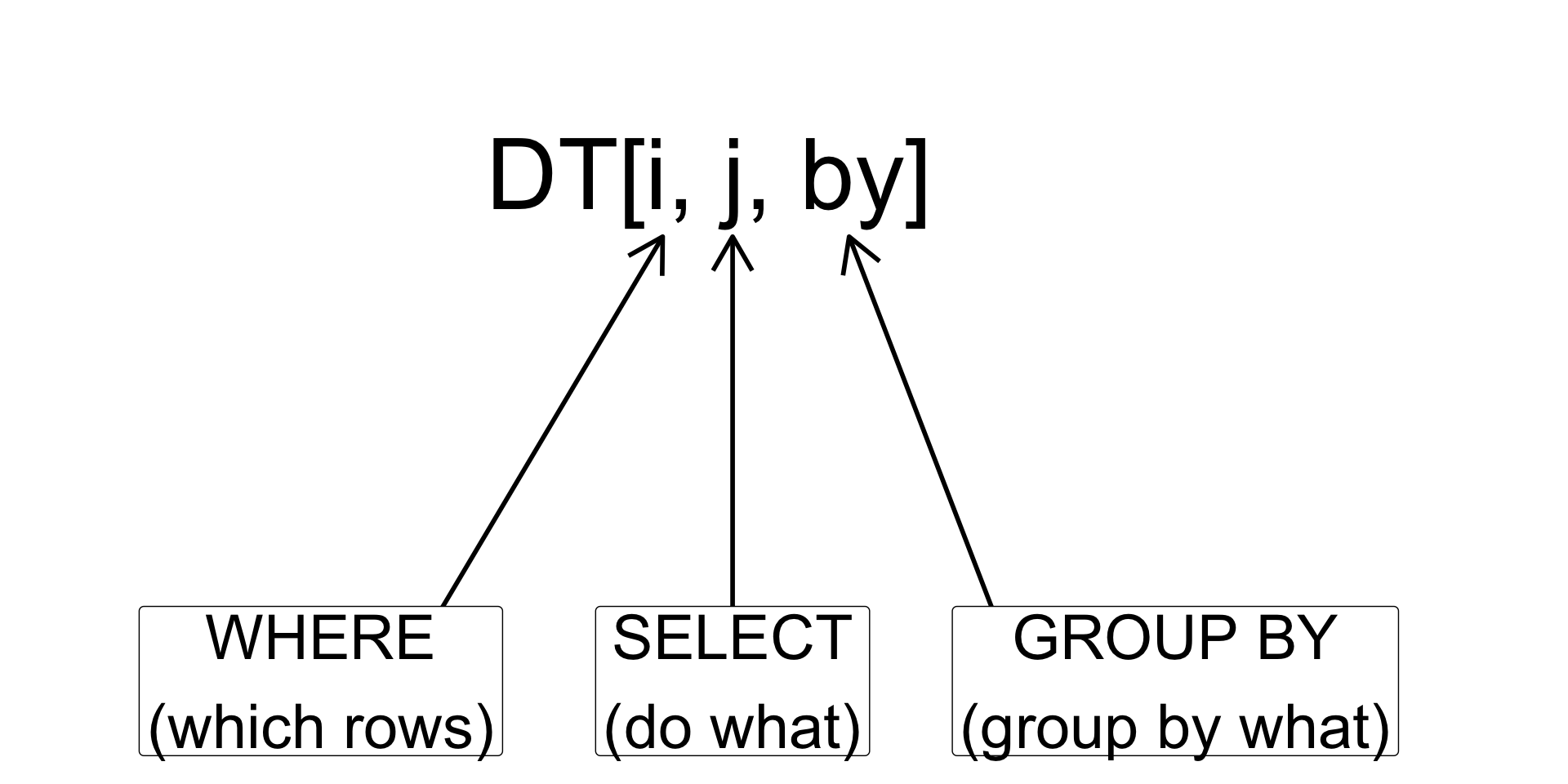
So, why should you use data.table?
- concise and consistent syntax
DT[i, j, by]
- speed
- faster than base R and
dplyr
- faster than base R and
- efficient memory usage
- sub-assign by reference:
DT[x < 0, y := NA] - aggregate while joining:
DT1[DT2, list(z=sum(z)), by = .EACHI](equivalent toDT1[, .(z=sum(z)), keyby=.(x,y)][DT2])
- sub-assign by reference:
- features
fread,fwrite, automatic indexing, rolling joins,foverlaps, etc.
More detail, here.
References
- Matt Dowle and Arun Srinivasan (2018).
data.table: Extension ofdata.frame. R package version 1.11.4. https://CRAN.R-project.org/package=data.table - https://github.com/Rdatatable/data.table/wiki
data.tablevs.dplyr. https://stackoverflow.com/questions/21435339/data-table-vs-dplyr-can-one-do-something-well-the-other-cant-or-does-poorly- Advaned tips and tricks with
data.table. http://brooksandrew.github.io/simpleblog/articles/advanced-data-table/ data.tablecheat sheet. https://s3.amazonaws.com/assets.datacamp.com/img/blog/data+table+cheat+sheet.pdf- Purpose of setting a key in
data.table. https://stackoverflow.com/questions/20039335/what-is-the-purpose-of-setting-a-key-in-data-table .EACHIindata.table. https://stackoverflow.com/questions/27004002/eachi-in-data-table/27004566#27004566- Understand
data.tablerolling joins. https://www.r-bloggers.com/understanding-data-table-rolling-joins/